Load arbitrary pulse shapes via spectrum and phase

[tinolang]

%example how to load arbitrary temporal pulse shapes as input pulse by using
%spectrum and phase
    
obj=chi3D('tag','arbitary temporal pulse shape'); 

obj('Nt',2^13,'tWindow',5e-12 ...
    ,'shiftFreqWindow',3e8/2e-6 ...
    ,'inloopFun','obj.userData(Etxy_o,Etxy_e,obj)' ...
    );

obj.userData = @(Eftfxfy_e,Eftfxfy_o,obj) plotPulseShape(Eftfxfy_e,Eftfxfy_o,obj); 

%% spectrum and phase for arb. temporal pulse shape


[Wavelength Spectrum Phase] = arbPulse(obj); % spectrum and phase for a pulse shape


Spectrum = obj.interpSpectrum(Wavelength,Spectrum);
Phase    = obj.interpPhase(Wavelength,Phase);

[Eftfxfy_fund Eftfxfy_sh]=obj.run({'pulse1' ...
    ,'EorI', 50e13 ...
    ,'material','Vacuum' ...
    ,'propagationLength',1e-3 ...
    ,'Spectrum',Spectrum ...
    ,'Phase',Phase });



function plotPulseShape(Etxy_e,Etxy_o,obj)
    %% plot pulse shapes
    It_o = sum(sum(abs(Etxy_o),3),2).^2;
    It_e = sum(sum(abs(Etxy_e),3),2).^2;

    figure(12)

    plot(obj.constVect.t,It_o/max(It_o(:)) ...
        ,obj.constVect.t,It_e/max(It_e(:)));
    xlim([-0.5e-12 0.5e-12])
    xlabel('time (s)')
    ylabel('intensity (norm)')
    legend({'fund';'sh'})


end


function [Wavelength Spectrum Phase]=arbPulse(obj)
%%
    lamc = 1e-6;
    
    sigma = 300e-15; % Width of the pulse
    Nt=obj.simProp.Nt;% 2^13;
    dt = obj.simProp.tWindow/(Nt-1)
%     dt=1e-15;
    t = linspace(-Nt/2*dt, Nt/2*dt, Nt)-dt/2;
    n = 10; % Order of the supergaussian
    
    % Supergaussian Pulse
    It = exp(-(abs(t)/sigma).^(2*n)) ...
        +1/2*exp(-(abs(t)/sigma*2).^(2*n)) ...
        -1/3*exp(-(abs(t)/sigma*5).^(2*n));
    
    
    
    F=(Nt-1)*dt
    df=1/F;
%     freq = linspace(-(Nt+1)*df,(Nt-1)*df,Nt)/2+ 3e8/lamc;
    freq = linspace(0,(Nt-1)*df,Nt)+obj.simProp.shiftFreqWindow;
    
    Ef = ifft(fftshift(sqrt(It).*exp(-1i*2*pi*(3e8/lamc-obj.simProp.shiftFreqWindow)*t)));
    If = abs(Ef).^2;
    Ph = phase(Ef);
    
    lam = 3e8./linspace(freq(end),freq(1),Nt);
    Ilam = interp1(3e8./freq,If,lam);
    Ilam = Ilam ./ lam.^2;
    Ilam = Ilam./max(Ilam(:));
    
    Phlam = interp1(3e8./freq,Ph,lam);

    lam_max =obj.constVect.lambda(1);
    lam_min =obj.constVect.lambda(end);
    Wavelength = lam(lam>lam_min & lam<=lam_max);
    Spectrum   = Ilam(lam>lam_min & lam<=lam_max);
    Phase      = Phlam(lam>lam_min & lam<=lam_max);  

    
    
    

    neq_ft = 3e8./(Wavelength);
    
    ft2 = linspace(min(neq_ft), max(neq_ft), length(neq_ft));  % linearized frequency grid
    If2 = interp1(fliplr(neq_ft),fliplr(Spectrum),ft2); % flip is needed: x data has to be monotonous
    If2 = If2./ft2.^2;
    If2 = If2/max(If2(:));
    
    Phase2 = interp1(fliplr(neq_ft),fliplr(Phase),ft2);

    Et2 = fftshift(ifft(sqrt(If2).*exp(1i*Phase2)));
    It2 = abs(Et2).^2; 
    dt2 = 1/diff(ft2([1 end]));
    Nt2 = length(ft2);
    t2 = linspace(-Nt2/2*dt2, Nt2/2*dt2, Nt2)-dt2/2;

    

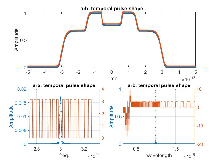
    % Plotting
        figure(10);
        subplot(2,2,[1 2])
        plot(t, It./max(It(:)),'.-' ...
            ,t2, It2./max(It2)+0.02,'.-');

        xlim([-0.5e-12 0.5e-12])
        xlabel('Time');
        ylabel('Amplitude');
        title('arb. temporal pulse shape');
        
        
        subplot(2,2,3)
        yyaxis left
        plot(freq,If,'.-');
        xlabel('freq.');
        ylabel('Amplitude');
        title('arb. temporal pulse shape');
        xlim(3e8./fliplr([.9e-6 1.1e-6]))
        yyaxis right
        plot(freq,Ph)
        grid on;   
    
        subplot(2,2,4)
        yyaxis left
        plot(lam,(Ilam),'.-');
        xlabel('wavelength');
        ylabel('Amplitude');
        title('arb. temporal pulse shape');
        xlim([lam_min lam_max])
        yyaxis right
        plot(lam,Phlam)
        grid on;
        
 



end