Calculating the M² Beam Parameter from Simulation Results

[tinolang]

Calculating the M² Beam Parameter from Simulation Results

In this post, I will walk through the steps required to calculate the M² beam quality factor from simulation results using data obtained from beam propagation through focus. The M² parameter is an important factor for characterizing the quality of laser beams, especially when comparing how closely the beam approximates an ideal Gaussian profile.

Simulation Setup

First, we set up a 3D simulation to propagate the beam through a focus. In this setup, the key parameters such as the propagation length, material, and beam radii in the x and y directions are defined. The detector captures the caustic of the beam, which is necessary to calculate the beam waist and Rayleigh range from which the M² is determined.

        % Initialize the simulation object
        obj = chi3D('tag', 'M2 fit');

        % Clear previous detectors and results
        obj.removeDetectors('all');
        obj.detectors.caustic.plotIntegratedProfiles=1;
        obj.clearResults;

        % Define the propagation through focus
        obj.run({'pulse1', ...
                 'propagationLength', 1, ...
                 'material', 'Air', ...
                 'eoo', 0, ...
                 'Nz', 25, ...
                 'showResultEach', 1, ...
                 'radiusOfCurvature_x', 0.5, ...
                 'radiusOfCurvature_y', 0.4, ...
                 'xWindow', 5e-3, ...
                 'yWindow', 5e-3, ...
                 'beamRadius_x', 0.4e-3, ...
                 'beamRadius_y', 0.5e-3, ...
                 'beamShape_x', {'supergauss', [5]} ...
               });
    

Extracting and Fitting the Data

After running the simulation, we extract the beam propagation data. This data contains the beam diameters in the x and y directions, and the propagation distances. From this, we calculate the beam radii by dividing the diameters by 2.

        % Measured data for beam propagation in x and y directions
        z = obj.simResults.caustic.z;  % Propagation distances
        radius_x = obj.simResults.caustic.diameter2M_x / 2;  % Beam radius in x-direction
        radius_y = obj.simResults.caustic.diameter2M_y / 2;  % Beam radius in y-direction

        % Center wavelength
        lambda_0 = obj.simResults.caustic.centerWavelength(end);  % Laser wavelength
    

Beam Propagation Model and Fitting

The beam propagation is modeled using the equation:

w(z) = w₀ * sqrt(1 + ((z - z₀) / zR)²)

Here, w(z) is the beam radius at a distance z from the beam waist, w₀ is the beam waist radius, z₀ is the location of the waist, and zR is the Rayleigh range. We use nonlinear least squares fitting to fit the measured data to this model, which allows us to extract w₀, z₀, and zR for both x and y directions.

        % Define the beam propagation model: w(z) = w_0 * sqrt(1 + ((z - z_0) / z_R)^2)
        beamRadiusModel = @(params, z) params(1) * sqrt(1 + ((z - params(2)) / params(3)).^2);

        % Initial guesses for the fit parameters (x and y)
        initialGuess_x = [min(radius_x), mean(z), (max(z) - min(z)) / 2];
        initialGuess_y = [min(radius_y), mean(z), (max(z) - min(z)) / 2];

        % Perform the fit using nonlinear least squares for both x and y directions
        options = optimset('TolFun', 1e-9, 'MaxIter', 1000);
        fitParams_x = lsqcurvefit(beamRadiusModel, initialGuess_x, z, radius_x, [], [], options);
        fitParams_y = lsqcurvefit(beamRadiusModel, initialGuess_y, z, radius_y, [], [], options);
    

Calculating the M² Parameter

After fitting the model, we can calculate the M² parameter using the formula:

M² = (π * w₀²) / (λ * zR)

This calculation is performed for both the x and y directions based on the fitted parameters w₀ and zR.

        % Extract fitted parameters and calculate M² for x and y directions
        w0_x = fitParams_x(1);  % Beam waist radius in x
        zR_x = fitParams_x(3);  % Rayleigh range in x
        M2_x = (pi * w0_x^2) / (lambda_0 * zR_x);  % M² for x-direction

        w0_y = fitParams_y(1);  % Beam waist radius in y
        zR_y = fitParams_y(3);  % Rayleigh range in y
        M2_y = (pi * w0_y^2) / (lambda_0 * zR_y);  % M² for y-direction
    

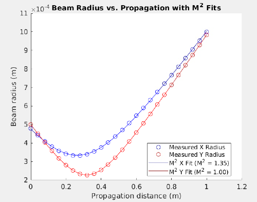
Plotting the Results

Finally, we plot the measured data points along with the respective fitted curves for both the x and y directions. The plots also show the calculated M² values.

        % Generate fitted curves
        fit_x = beamRadiusModel(fitParams_x, z);
        fit_y = beamRadiusModel(fitParams_y, z);

        % Plot the results
        figure;
        hold on;

        % Plot measured data points and fitted curves for x and y directions
        plot(z, radius_x, 'bo', 'DisplayName', 'Measured X Radius');
        plot(z, radius_y, 'ro', 'DisplayName', 'Measured Y Radius');
        plot(z, fit_x, 'b-', 'DisplayName', sprintf('M^2 X Fit (M^2 = %.2f)', M2_x));
        plot(z, fit_y, 'r-', 'DisplayName', sprintf('M^2 Y Fit (M^2 = %.2f)', M2_y));

        % Set labels, title, and legend
        xlabel('Propagation distance (m)');
        ylabel('Beam radius (m)');
        legend('Location', 'best');
        title('Beam Radius vs. Propagation with M^2 Fits');

        hold off;
    

Conclusion

This method provides an accurate way to extract the beam quality factor M² from the simulated beam propagation data. By fitting the measured data to the beam propagation model, we can determine the beam waist, Rayleigh range, and the M² value for both the x and y directions.